Diagnostic of assessments in MSE: did Assess models converge during MSE?

Diagnostic check for convergence of Assess models during closed-loop simulation. Use when the MP was created with make_MP with argument diagnostic = "min" or "full". This function summarizes and plots the diagnostic information.

Usage

diagnostic(MSE, MP, gradient_threshold = 0.1, figure = TRUE)

diagnostic_AM(...)

Arguments

MSE: An object of class MSE created by MSEtool::runMSE().
MP: Optional, a character vector of MPs that use assessment models.
gradient_threshold: The maximum magnitude (absolute value) desired for the gradient of the likelihood.
figure: Logical, whether a figure will be drawn.
...: Arguments to pass to diagnostic.

Value

A matrix with diagnostic performance of assessment models in the MSE. If figure = TRUE, a set of figures: traffic light (red/green) plots indicating whether the model converged (defined if a positive-definite Hessian matrix was obtained), the optimizer reached pre-specified iteration limits (as passed to stats::nlminb()), and the maximum gradient of the likelihood in each assessment run. Also includes the number of optimization iterations function evaluations reported by stats::nlminb() for each application of the assessment model.

Author

Q. Huynh

Examples

# \donttest{
OM <- MSEtool::testOM; OM@proyears <- 20
myMSE <- runMSE(OM, MPs = "SCA_4010")
#> ℹ Checking OM for completeness
#> ✔ Loading operating model
#> ✔ Optimizing for user-specified movement
#> ✔ Calculating MSY reference points for each year
#> ✔ Optimizing for user-specified depletion in last historical year
#> ✔ Calculating historical stock and fishing dynamics
#> ✔ Calculating per-recruit reference points
#> ✔ Calculating B-low reference points
#> ✔ Calculating reference yield - best fixed F strategy
#> ✔ Simulating observed data
#> ✔ Running forward projections
#> ✔ 1 / 1  Running MSE for SCA_4010 
#> 
  |===                                               | 5 % ~21s          
  |======                                            | 11% ~10s          
  |========                                          | 16% ~06s          
  |===========                                       | 21% ~04s          
  |==============                                    | 26% ~07s          
  |================                                  | 32% ~05s          
  |===================                               | 37% ~04s          
  |======================                            | 42% ~03s          
  |========================                          | 47% ~04s          
  |===========================                       | 53% ~03s          
  |=============================                     | 58% ~03s          
  |================================                  | 63% ~02s          
  |===================================               | 68% ~03s          
  |=====================================             | 74% ~02s          
  |========================================          | 79% ~02s          
  |===========================================       | 84% ~01s          
  |=============================================     | 89% ~01s          
  |================================================  | 95% ~00s          
  |==================================================| 100% elapsed=08s  
#> 
diagnostic(myMSE)
#> ✔ Creating plots for MP:
#>   SCA_4010

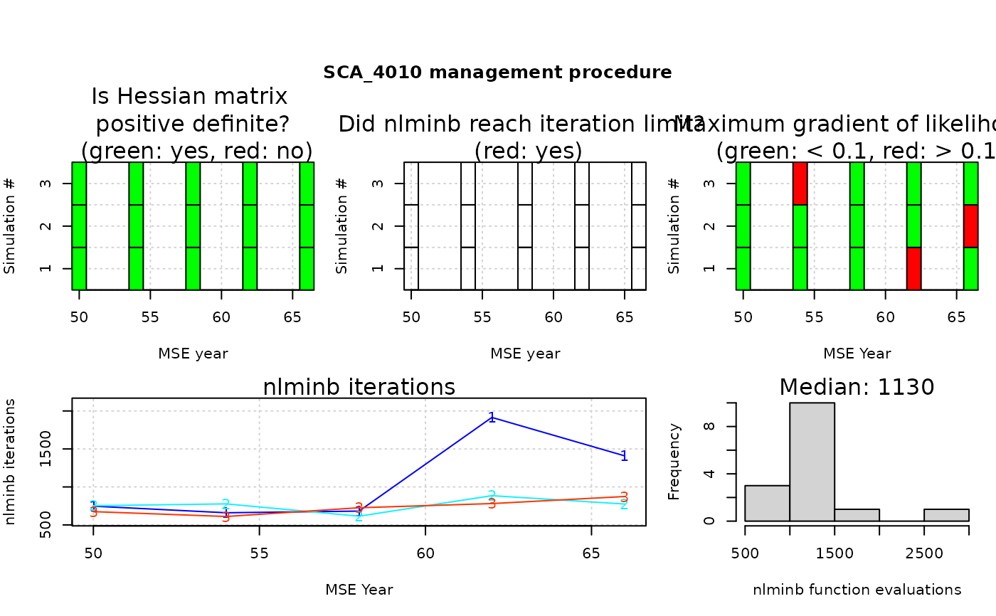#>                                   SCA_4010
#> Percent positive-definite Hessian      100
#> Percent iteration limit reached          0
#> Percent max. gradient < 0.1             80
#> Median iterations                      753
#> Median function evaluations           1130

# How to get all the reporting
library(dplyr)
#> 
#> Attaching package: ‘dplyr’
#> The following objects are masked from ‘package:stats’:
#> 
#>     filter, lag
#> The following objects are masked from ‘package:base’:
#> 
#>     intersect, setdiff, setequal, union
conv_statistics <- lapply(1:myMSE@nMPs, function(m) {
  lapply(1:myMSE@nsim, function(x) {
    myMSE@PPD[[m]]@Misc[[x]]$diagnostic %>%
      mutate(MP = myMSE@MPs[m], Simulation = x)
 }) %>% bind_rows()
}) %>% bind_rows()
# }